Mapping with ggplot2 and sf

Have you ever made a map in ArcGIS, only to later realize that you made a mistake with your data and will have to remake the entire thing? That’s where the sf package in R comes in!

Let’s load the sf and tidyverse packages.

# Uncomment and run this only once
#install.packages("sf")
library(sf)
library(tidyverse)

Now, we’ll need to load our data. We’ll use the North Carolina counties data built into the sf package.

nc <- st_read(system.file("shape/nc.shp", package = "sf"))

Reading layer `nc' from data source 
  `/Library/Frameworks/R.framework/Versions/4.4-arm64/Resources/library/sf/shape/nc.shp' 
  using driver `ESRI Shapefile'
Simple feature collection with 100 features and 14 fields
Geometry type: MULTIPOLYGON
Dimension:     XY
Bounding box:  xmin: -84.32385 ymin: 33.88199 xmax: -75.45698 ymax: 36.58965
Geodetic CRS:  NAD27

Every sf object has a “geometry” column, which stores the coordinates of the point, line, or polygon. Now, let’s plot it. The ggplot2 package has a geom_sf option for simple features.

ggplot() + geom_sf(data = nc)

# if that does not work, you may have to specify the geometry in the aesthetic
ggplot() + geom_sf(data = nc, aes(geometry = geometry))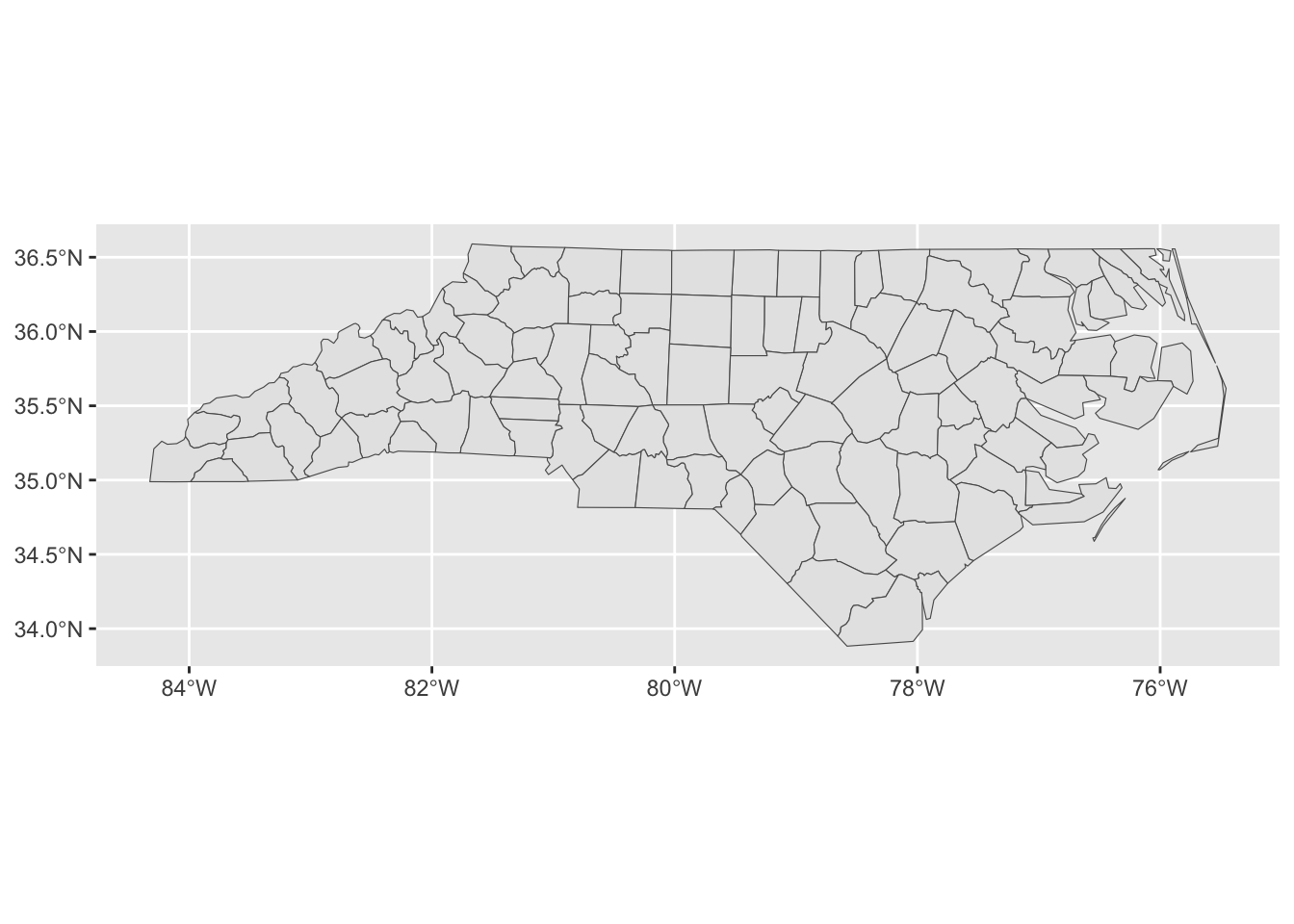

Not bad. I prefer to not see the latitude/longitude along the axes, so I frequently use theme_void().

ggplot() + geom_sf(data = nc) + theme_void()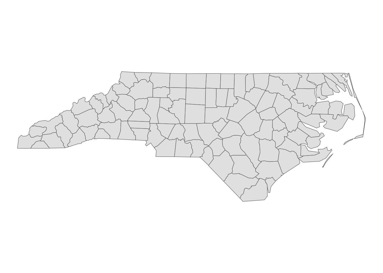

Great! This dataset has several attributes related to births and infant deaths. We’ll use the SID79, which is the number of sudden infant deaths in the year 1979 for each county.

ggplot() + geom_sf(data = nc, aes(fill = SID79)) + theme_void()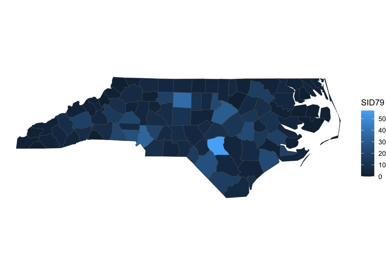

The ggplot default colors are not my favorite. I prefer using brewer colors. The direction argument reverses the direction of color darkening so that darker indicates a higher value.

ggplot() + geom_sf(data = nc, aes(fill = SID79)) + theme_void() +
  scale_fill_distiller(palette = "YlOrBr", direction = 1)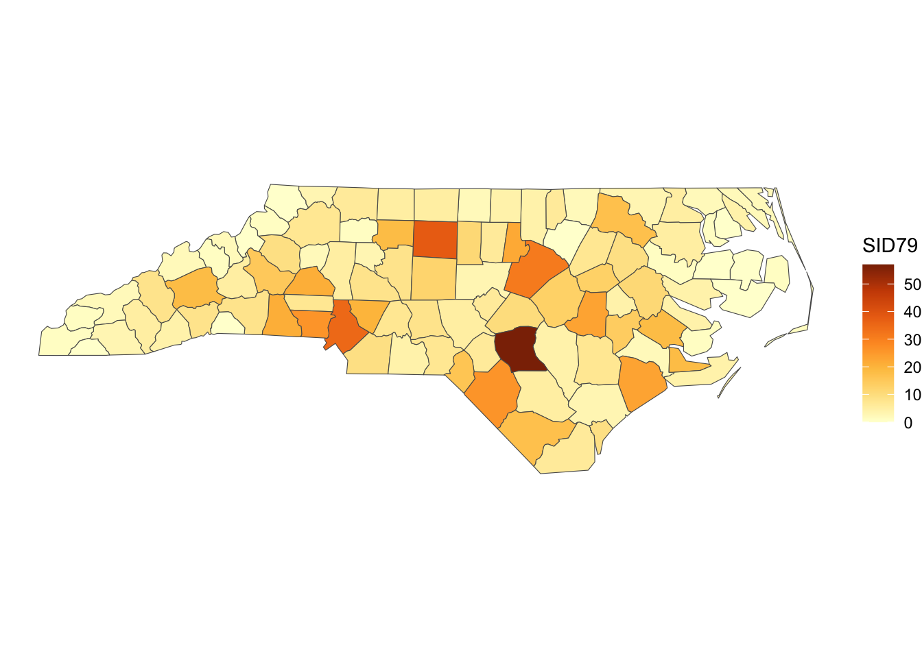

We can see quite clearly that a few counties in central North Carolina had a large number of sudden infant deaths in 1979. To clean up this map, let’s add a scale bar and north arrow (using the ggspatial package), and refine the labels.

library(ggspatial)

ggplot() +
  geom_sf(data = nc, aes(fill = SID79)) +
  theme_void() +
  scale_fill_distiller(palette = "YlOrBr", direction = 1) +
  annotation_scale(location = "bl", line_width = 1) +
  annotation_north_arrow(style = north_arrow_fancy_orienteering(),
                         location = "tl", 
                         height = unit(0.8, "cm"),
                         width = unit(0.8, "cm")) +
  labs(fill = "SIDS 1979")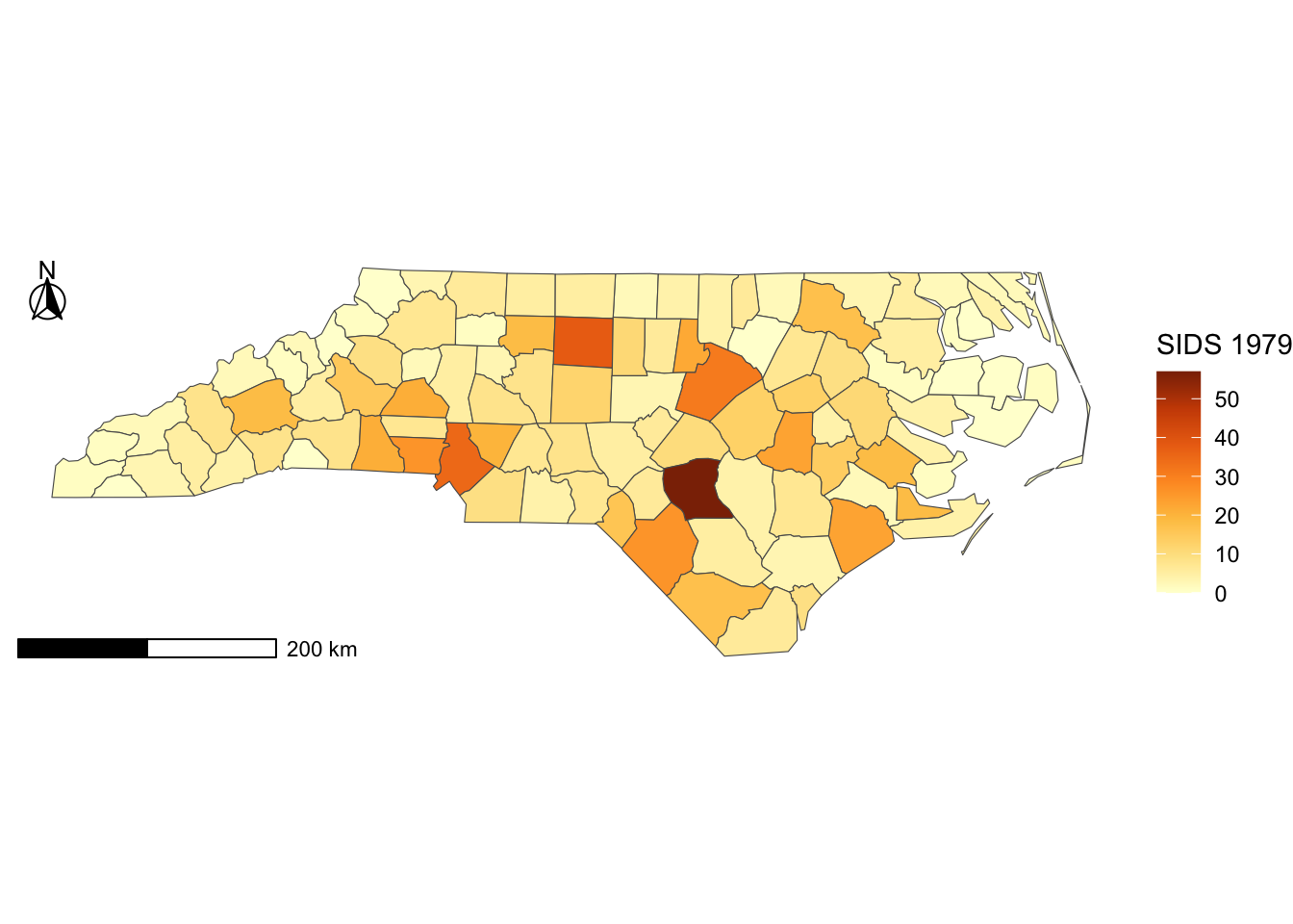

Much better! The scale bar and north arrow size can be adjusted as needed. This mostly depends on how large you save the figure. These ggplot objects can be saved the same way as a regular plot.

ggsave("nc.jpg", width = 5, height = 3, dpi = 300)

And you’re done! You’ve created your first official map in R!

Thanks for joining me. Keep an eye out for more tutorials in R!

Subscribe